Flashcards for Reiner Pope on Dwarkesh Podcast

$T = \max(t_{\text{compute}},\ t_{\text{mem}})$

$t_{\text{compute}} = \frac{B \cdot N_{\text{active}}}{\text{FLOPs}}$

where $B$ is batch size, $N_{\text{active}}$ is active parameters, and FLOPs is the compute throughput of the hardware.

$t_{\text{mem}} = \frac{N_{\text{total}} + B \cdot \text{len}_{\text{ctx}} \cdot \text{KV}_{\text{bytes/token}}}{\text{mem\_bw}}$

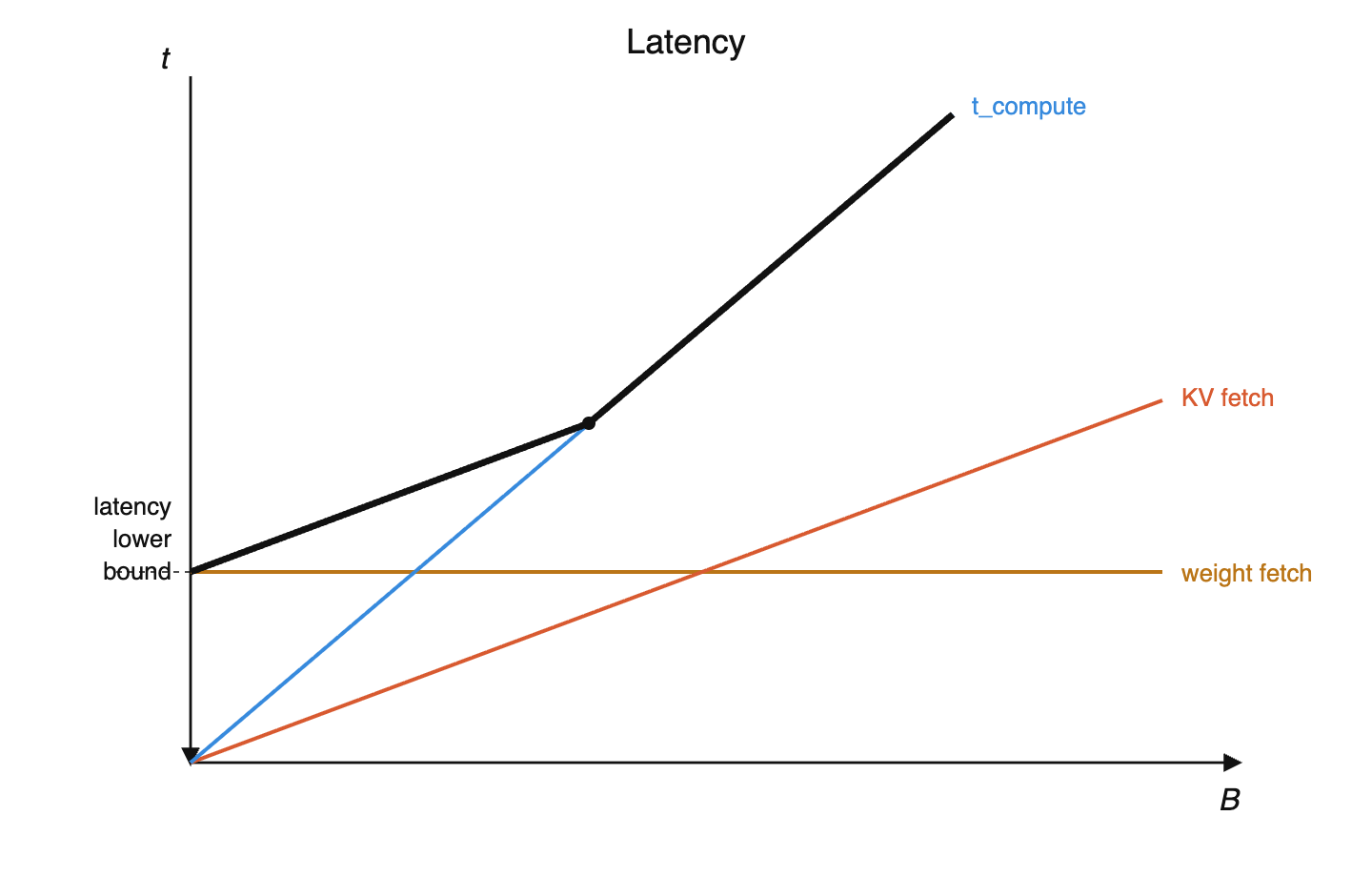
Because you still have to load all the active parameters into memory.

Compute time, and memory time for KV cache fetches, cannot be amortized with batch size.

$\sim 300$ FLOPs / byte.

Set compute time = memory time (at equality, both resources are fully saturated):

$\frac{B \cdot N_{\text{active}}}{\text{FLOPs}} = \frac{N_{\text{total}}}{\text{mem\_bw}}$

Solve for $B$:

$B = \frac{\text{FLOPs}}{\text{mem\_bw}} \cdot \frac{N_{\text{total}}}{N_{\text{active}}} = 300 \cdot \frac{1}{\text{sparsity}}$

So $B \geq 300 / \text{sparsity}$.

Why: compute scales with $B$ (each token needs its own matmul), but weight fetches don't (load once, reuse across batch). Need enough tokens to amortize the fetch.

DeepSeek V3: $32/256$ active → $B \geq 300 \times 8 = 2{,}400$.

20ms is the HBM drain time — memory capacity ÷ memory bandwidth. E.g. Rubin: $288\text{ GB} / 20\text{ TB/s} \approx 15\text{ms}$.

Faster than 20ms is impossible because you physically can't read all the weights from HBM in less time than bandwidth allows.

Slower than 20ms means you're just leaving the FLOPs idle, because there's nothing left to read.

MoE communication is all-to-all (any GPU's tokens may route to any other GPU's experts).

Within a rack, NVLink connects every GPU to every other at full bandwidth, which is a perfect fit for all-to-all. Across racks, scale-out is $\sim 8\times$ slower and bottlenecks the all-to-all.

At the beginning of the batch, the GPUs dedicated to the final layers are not being used, and conversely at the end of the batch, the GPUs dedicated to the first layers are not being used.

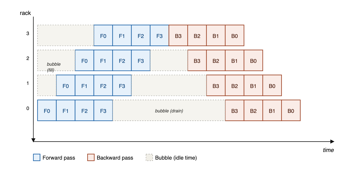
You need to consolidate gradients and update the model before you process the next batch.

Keeping $P$ stages busy requires $P$ micro-batches in flight, so concurrent sequences scale with $P$.

Given that KV cache often dominates memory at long context lengths, pipelining's value is limited.

You're adding architecture constraints — things like Kimi's attention-to-residuals (where each block attends to all previous layers' residuals) become very difficult when those residuals live on different pipeline stages. Similarly, interleaving sliding-window and global attention layers could cause load imbalance across stages. Dealing with all this slows down research iteration, which is the greatest sin you can commit.

2 FLOPs per parameter per token for the forward pass (multiply + add). Backward pass is $2\times$ forward because you compute gradients w.r.t. both input matrices. So $2 + 4 = 6$.

$C_{\text{total}} = C_{\text{pretrain}} + C_{\text{RL}} + C_{\text{inference}}$

$C_{\text{pretrain}} = 6 \times N_{\text{active}} \times D_{\text{pretrain}}$ (the $6ND$ formula — forward + backward)

$C_{\text{RL}} = (2 \text{ to } 6) \times N_{\text{active}} \times D_{\text{RL}} \times \text{inefficiency}$ (2 if you don't train on the rollout and do forward only, up to 6 if you do; inefficiency from low MFU during decode)

$C_{\text{inference}} = 2 \times N_{\text{active}} \times D_{\text{inference}} \times \text{inefficiency}$ (forward pass only; lower MFU during decode)

If pre-training, RL, and inference costs trade off (more pre-training → less RL/inference needed for same quality, and vice versa), the optimum is approximately where all three are equal.

$6 \times D_{\text{pretrain}} = 3 \times D_{\text{RL}} \times 3 \times \text{inefficiency} = 2 \times D_{\text{inference}} \times 3 \times \text{inefficiency}$

$D_{\text{pretrain}} = 1.5\, D_{\text{RL}} = D_{\text{inference}}$

$D_{\text{inference}} \approx 50\text{M tokens/sec} \times 60\text{ days} \times 86{,}400\text{ sec/day} \approx 200\text{T tokens}$

$D_{\text{pretrain}} \approx D_{\text{inference}} \approx 200\text{T tokens}$

$D_{\text{chinchilla}} \approx 20 \times 100\text{B} = 2\text{T tokens}$

$200\text{T} / 2\text{T} = 100\times$

Below this point, you're compute bound, whose cost is flat as context length increases.

Above this point, you're memory time bound, thanks to KV cache growing, and that increases linearly with context length.

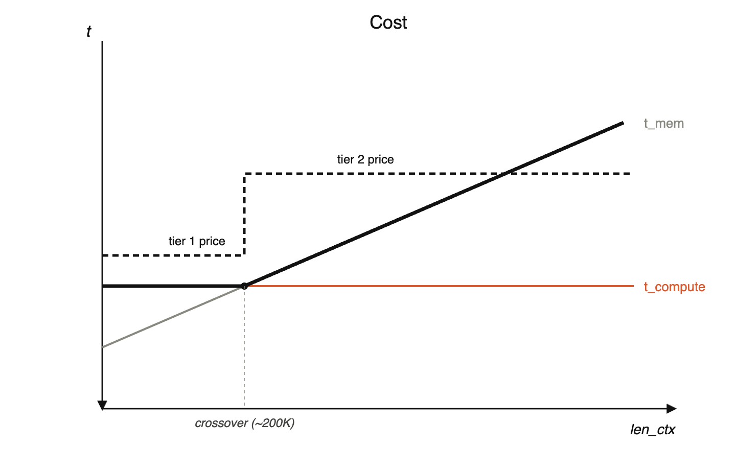
At the crossover, $t_{\text{compute}} = t_{\text{KV fetch}}$:

$\frac{B \cdot N_{\text{active}}}{\text{FLOPs}} = \frac{B \cdot \text{len}_{\text{ctx}} \cdot \text{bytes/token}}{\text{mem\_bw}}$

Solve for bytes/token:

$\text{bytes/token} = \frac{\text{mem\_bw}}{\text{FLOPs}} \cdot \frac{N_{\text{active}}}{\text{len}_{\text{ctx}}} = \frac{1}{300} \cdot \frac{N_{\text{active}}}{\text{len}_{\text{ctx}}}$

Plug in: $N_{\text{active}} \approx 100\text{B}$, $\text{len}_{\text{ctx}} = 200\text{K}$ → $\text{bytes/token} \approx 1.7\text{ KB}$.

MFU during decode is about $\tfrac{1}{5}$ that during prefill.

This is because in prefill, you're processing the whole sequence in parallel, so the weight fetch can be amortized across lots of compute, whereas in decode, you have to load all the weights in just to process one more token, which means you're wasting FLOPs while you're waiting for the weights to show up from memory.

Loading KVs from memory is much cheaper than recomputing.

They've both had this convergent evolution where cryptographic protocols need every output bit to depend on every input bit in complicated ways, and similarly, NNs need output to make connections between inputs.

Cryptographic protocols take something which has a lot of structure and make it seem indistinguishable from random. Whereas NNs take something which may look random and extract structure from it.